
X.C. Mol* Protein–Protein Interface
Didem Vardar-Ulu; Youngjoo Kim; and Shane Austin
Overview: This activity demonstrates how to display interactions at the interface of two macromolecules.
Outcome: The user will be able to display contacts at the interface of two macromolecules and display the non-covalent interactions stabilizing the interface.
Time to complete: 20-25 minutes
Modeling Skill
- Display contacts at a protein-protein interface
About the Model
PDB ID: 6m0j
Protein: SARS-CoV-2 spike receptor-binding domain bound to the ACE2 receptor
Activity: Angiotensin-converting enzyme 2 (Chain A); Spike protein S1 (Chain B); NAG–glycan; Zn2+; Cl–
Description: Receptor for the pandemic virus, SARS-CoV-2
Steps
Load the Structure:
- Go to rcsb.org
- In the search bar at the top, type 6m0j and press Enter.
- On the landing page, click the “Structure” tab next to the highlighted “Structure Summary” tab to open the user interface and load the structure.
Create separate components for Angiotensin-converting enzyme 2 (Chain A) and Spike protein S1 (Chain B): (Figure 1)
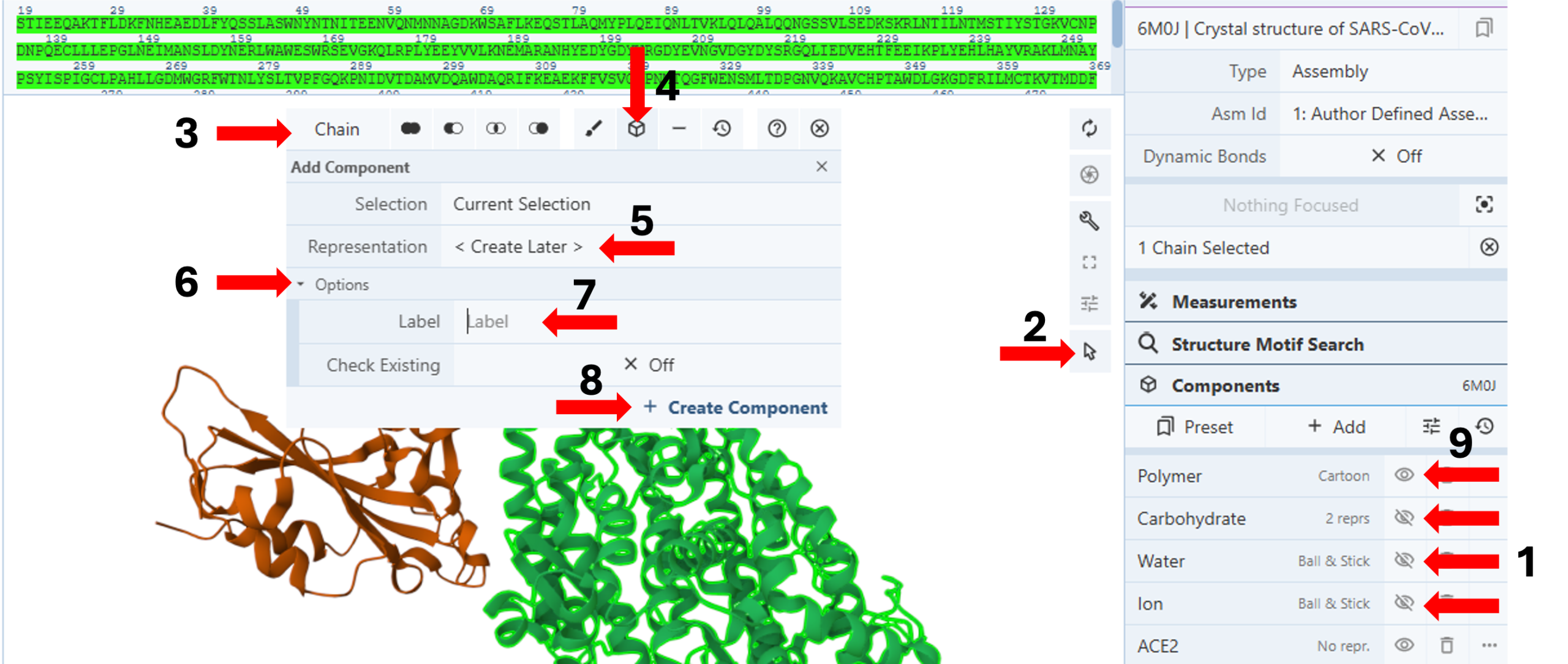
- To simplify the view on the 3D-canvas, use the “eye” icon in the components panel to hide the “carbohydrate,” “water,” and “ion” components. (Arrow 1)
- Activate the “Select Mode Toggle” by clicking the “cursor” icon. (Arrow 2)
- Choose your picking level as “Chain”. (Arrow 3)
- Click the chain you want to create a component for (e.g., Chain A).
- Click on the “Components Icon”. (Arrow 4)
- Keep the default “<Create Later>” for “Representation”. (Arrow 5)
- Click “Options”. (Arrow 6)
- Enter the desired component name (e.g., ACE2) next to the cell for “Label”. (Arrow 7)
- Click “Create Component”. (Arrow 8)
- Deselect Chain A (ACE2) by clicking the empty 3D canvas.
- Repeat steps 7-13 for Chain B (e.g., S1).
- Hide a polymer representation (Arrow 9).
Note: You will now have a blank 3D canvas since you opted to add representations later by selecting the default representation for the new component.
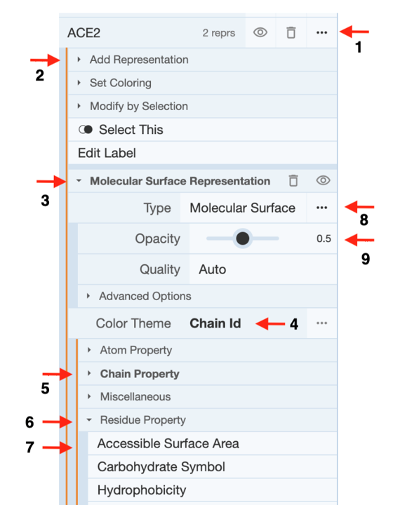
Show Accessible Surface Area using separate representations for ACE2 and Spike Protein: (Figure 2)
-
-
-
-
-
-
-
-
- Click the three dots next to “ACE2” in the components menu (Arrow 1).
- Click “Add representation” (Arrow 2) to activate the drop-down menu with available representations.
- Select “Molecular Surface”.
- Re-click “Add representation” (Arrow 2) to collapse the drop-down menu.
- Click “Molecular Surface Representation” for the drop-down menu. (Arrow 3)
- Click “Chain ID” next to “Color Theme” to access theme options. (Arrow 4)
- Click “Chain Property” to collapse the open menu. (Arrow 5)
- Click “Residue Property” to access property options. (Arrow 6)
-
-
-
-
-
-
-
-
- Click “Accessible Surface Area”. (Arrow 7)
- Click the three dots next to “Cartoon” (Arrow 8)
- Decrease the Opacity to 0.5 (Arrow 9)
- Click “Add representation” (Arrow 2) to activate the drop-down menu with available representations.
- Select “Cartoon Representation”.
- Re-click “Add representation” (Arrow 2) to collapse the drop-down menu.
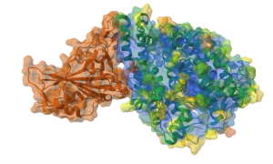
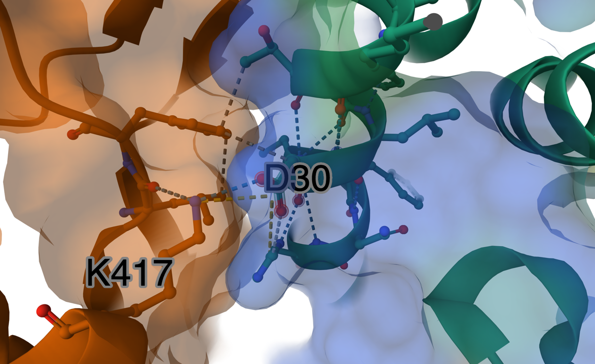
Figure 3. Semitransparent Molecular Surface Representation of molecular interface overlaying cartoon representation of the proteins (ACE2: green, S1: brown) - Repeat steps 16-29 for “S1”, but do not change the “Color Theme” in step 21. (Figure 3)
- Click the three dots next to ACE2 and S1 to collapse all dropdown menus.
- Change the “Picking Level” to “Residue”. (Figure 1, Arrow 3)
- Deactivate the “Select Mode Toggle” by clicking the “cursor” icon. (Figure 1, Arrow 2)

Displaying Residues and Interactions at the ACE2-S1 Interface:
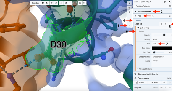
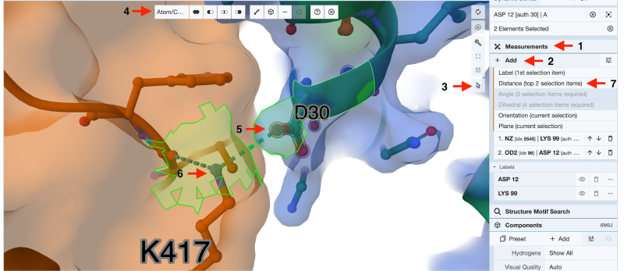
Show and Label Residues: (Figure 4)
- Click a residue from ACE2 at the ACE2-S1 interface using the sequence panel or the 3D canvas (e.g., D30), create the temporary components for the target (D30) and its 5Å surroundings. (See Chapter VII.C)
- Label this residue.
-
- Activate the “Select Mode Toggle” by clicking the “cursor” icon.
- Click D30 to select and highlight it in green. (Arrow 1)
- Click “Measurements” to expand the menu. (Arrow 2)
- Click “Add”. (Arrow 3)
- Click “Labels”. (Arrow 4)
- Click the three dots next to the current label “ASP12”. (Arrow 5)
- Click “Options”. (Arrow 6)
- Type the new label in the cell next to “Text”. (Ex: D30) (Arrow 7)
- Re-click the three dots next to the current label “ASP12” to collapse the label menu. (Arrow 5)
- Deselect residue D30 by clicking the empty 3D canvas.
- In the sequence panel, choose “Spike Protein S1”.
- Click K417 to select and highlight it in green.
- Repeat steps c-j and label the residue as “K417”.
Note: The numbering for the displayed label assumes the first residue of the sequence to be 1, which may not be the case for N-terminally truncated residues, as in this case. You can modify the label to display the label of your choice.
- Deactivate the “Select Mode Toggle” by clicking the “cursor” icon. (Arrow 1)
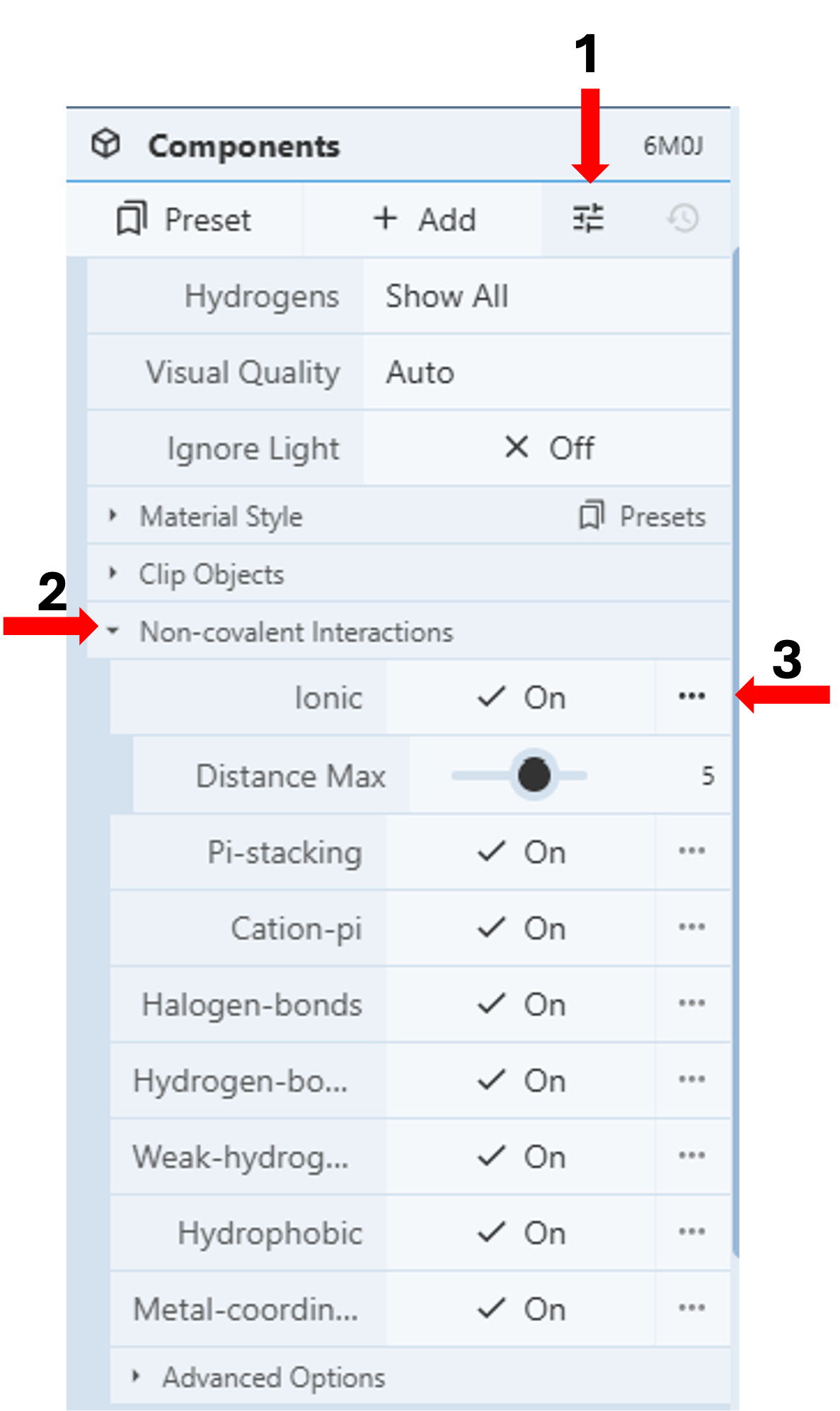
Show and Adjust Non-covalent Interactions: (Figure 5)
-
-
-
-
-
-
-
-
- Click the “Settings” icon in the first row under the Components Panel to access the pull-down menu. Figure 5 (Arrow 1)
- Click “Non-covalent Interactions” Figure 5 (Arrow 2)
- Turn on all the interactions by clicking the corresponding on/off toggle.
- Click the three dots next to any interaction to expand the menu for additional adjustments, such as interaction distance. Figure 5 (Arrow 3)
-
-
-
-
-
-
-
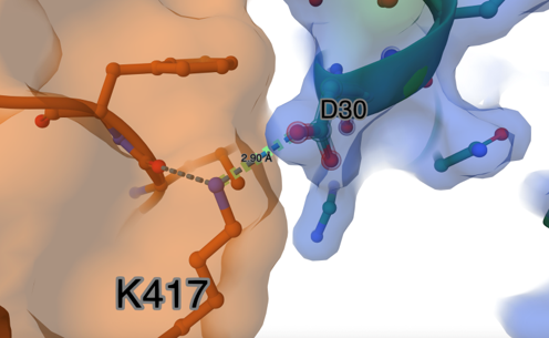
Show distance between D30 and K417: (Figure 7)
- To show only the interaction between D30 and K417, turn on “hydrogen-bonds” only and change “Don out of plane angle max” to zero.
- To show the distance between D30 and K417, click on the “Measurement” (Arrow 1) in the panel on the right, then “Add”. (Arrow 2)
- Activate the “toggle selection mode” by clicking the “cursor” icon. (Arrow 3)
- Choose your picking level as “Atom/Coarse Element”. (Arrow 4).
- Click on the oxygen atom of D30, which is hydrogen-bonded to K417. It will be labeled as number 1 initially, then change to number 2 when you click on the nitrogen atom in step 42. (Arrow 5)
- Click on the nitrogen atom in K417, which will now be labeled as number 1, and the oxygen atom will be labeled as number 2. (Arrow 6)
- Click on the “distance (top 2 selection items)” under the “Measurement” (Arrow 7).
- The final image with the distance between D30 and K417 is shown in Figure 8.
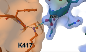
Figure 8. Labed distance between oxygen from D30 and nitrogen from K417.
Jump to the next Mol* tutorial: XI.C. Superimposition